Getting Started

This tutorial demonstrates the complete workflow of the mievformer package for microenvironmental analysis.

1. Setup and Data Loading

First, we load the necessary libraries and the dataset. We will use a subsampled version of the lung dataset for this tutorial.

import mievformer as mf
import scanpy as sc
import numpy as np
import os

# Path to the original data
original_data_path = "nichedynamics/data/20230629__230629pre/output-XETG00057__0003908__lung__20230629__073037/adata.h5ad"

# Load data
if os.path.exists(original_data_path):
    adata = sc.read_h5ad(original_data_path)
    print(f"Loaded data with {adata.shape[0]} cells and {adata.shape[1]} genes.")

    # Subsample to 10k cells for tutorial
    if adata.shape[0] > 10000:
        sc.pp.subsample(adata, n_obs=10000)
        print(f"Subsampled to {adata.shape[0]} cells.")
else:
    print(f"Data file not found at {original_data_path}. Please check the path.")
    # Create dummy data for testing if file not found
    adata = sc.AnnData(np.random.rand(10000, 100))
    adata.obsm['spatial'] = np.random.rand(10000, 2)
    adata.obsm['X_pca'] = np.random.rand(10000, 20)
    adata.obs['cell_type'] = np.random.choice(['TypeA', 'TypeB', 'TypeC'], 10000)
    print("Created dummy data.")

2. Optimize Mievformer Model

We optimize the Mievformer model to learn the niche representation. This step involves training a model to reconstruct the cellular neighborhood.

# Define model path
model_path = "tutorial_model.pth"

# Optimize model
# We use a small number of epochs for demonstration purposes
adata = mf.optimize_nicheformer(
    adata,
    model_path=model_path,
    max_epochs=10,  # Increase for real analysis
    batch_size=128,
    latent_dim=20,
    neighbor_num=100
)

print("Optimization complete.")
print("Added keys to adata.obsm:", adata.obsm.keys())

3. Calculate wb_ez

Calculate the weight and bias terms for the embedding. This step is required before calculating spatial distribution.

# Calculate wb_ez (required for spatial distribution)
adata = mf.calculate_wb_ez(adata, model_path)
print("Embedding 'e' shape:", adata.obsm['e'].shape)
print("Weights 'w_z' shape:", adata.obsm['w_z'].shape)

4. Niche Density Ratio and Cluster Membership

For each cell, compute the density ratio p(e|z)/p(e) over a panel of reference niches (softmax-normalized per cell), then aggregate by niche cluster to obtain a per-cell soft membership over niche clusters.

# Per-cell density ratio over reference niches
adata = mf.calculate_niche_density_ratio(adata)

# Aggregate into per-cell niche-cluster membership
adata = mf.calculate_niche_cluster_membership(adata)
print("Niche density ratio and cluster membership computed.")

5. Estimate Population Density

Estimate the density of specific cell populations.

# Check available cell types
print(adata.obs['cell_type'].unique())

# Estimate density for a specific group (e.g., the first one found)
target_group = adata.obs['cell_type'].unique()[0]
print(f"Estimating density for: {target_group}")

adata = mf.estimate_population_density(adata, group=target_group, cluster_key='cell_type')

print(f"Density estimated. Added '{target_group}_density' to adata.obs.")

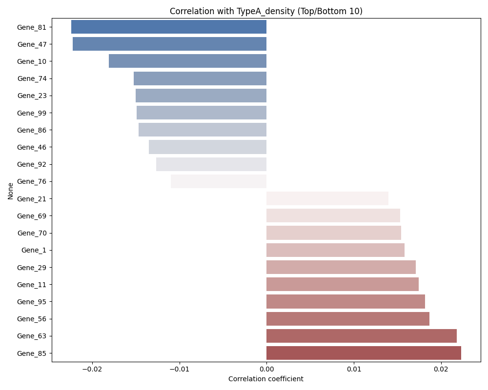
6. Analyze Density Correlation

Analyze the correlation between the estimated density and gene expression.

density_col = f'{target_group}_density'
output_plot = "density_correlation.png"

corrs = mf.analyze_density_correlation(
    adata,
    density_col=density_col,
    file_path=output_plot
)

print("Top 5 correlated genes:")
print(corrs.nlargest(5))

# Display the plot
# from IPython.display import Image
# if os.path.exists(output_plot):
#     display(Image(filename=output_plot))

# In the documentation build, we display the pre-generated image:

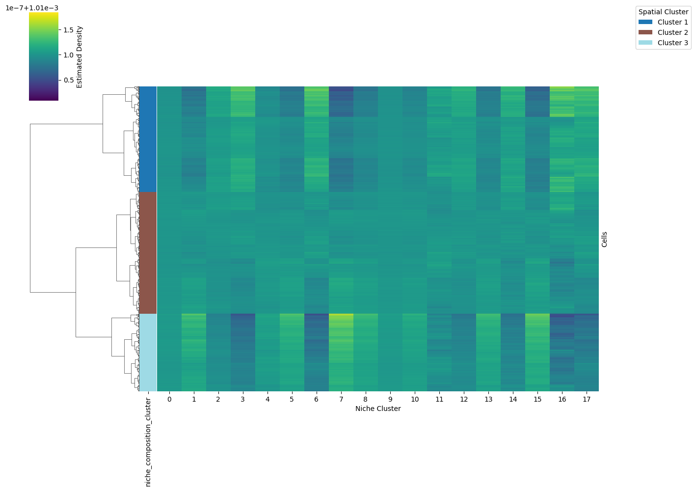
7. Analyze Niche Membership

Cluster cells by their niche-cluster membership vectors (obsm['dist_e_agg']) and visualize the membership matrix as a clustermap.

# Analyze niche membership
# Cluster cells using Ward hierarchical clustering on the niche-cluster
# membership vectors, and draw a clustermap.

if 'leiden_e' not in adata.obs:
    print("Running Leiden clustering on 'e' embedding...")
    sc.pp.neighbors(adata, use_rep='e')
    sc.tl.leiden(adata, key_added='leiden_e')

adata = mf.analyze_niche_membership(
    adata,
    n_clusters=3,  # Number of cell clusters based on niche membership
    file_path='niche_composition_clustermap.png'
)

print("Niche membership analysis complete.")
print("Added 'niche_composition_cluster' to obs:", 'niche_composition_cluster' in adata.obs)

# Display the plot
# from IPython.display import Image
# if os.path.exists('niche_composition_clustermap.png'):
#     display(Image(filename='niche_composition_clustermap.png'))

Summary

In this tutorial, we covered the complete Mievformer workflow:

1. Data Loading: Load and preprocess spatial transcriptomics data

2. Model Training: Use optimize_nicheformer to learn microenvironmental embeddings

3. Embedding Calculation: Use calculate_wb_ez to compute weight and bias terms

4. Niche Density Ratio and Membership: Use calculate_niche_density_ratio and calculate_niche_cluster_membership to compute per-cell p(e|z)/p(e) over reference niches and aggregate it into a per-cell niche-cluster membership

5. Density Estimation: Use estimate_population_density to estimate cell population density

6. Correlation Analysis: Use analyze_density_correlation to find correlated genes

7. Niche Membership Analysis: Use analyze_niche_membership to cluster cells by niche membership and visualize

For more details on each function, see the API Reference.